| Individual receiver of the Keck Array |
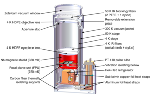 |
Figure 1: Individual receiver of the Keck Array. Each receiver
is cryogenic, with a pulse tube refrigerator cooling the
optics to 4 K and a three-stage sorption refrigerator cooling
the focal plane to 270 mK. The Keck Array consists of
five identical receivers on a single telescope mount at the
South Pole.
|
PDF / PNG |
| Observing time |
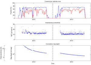 |
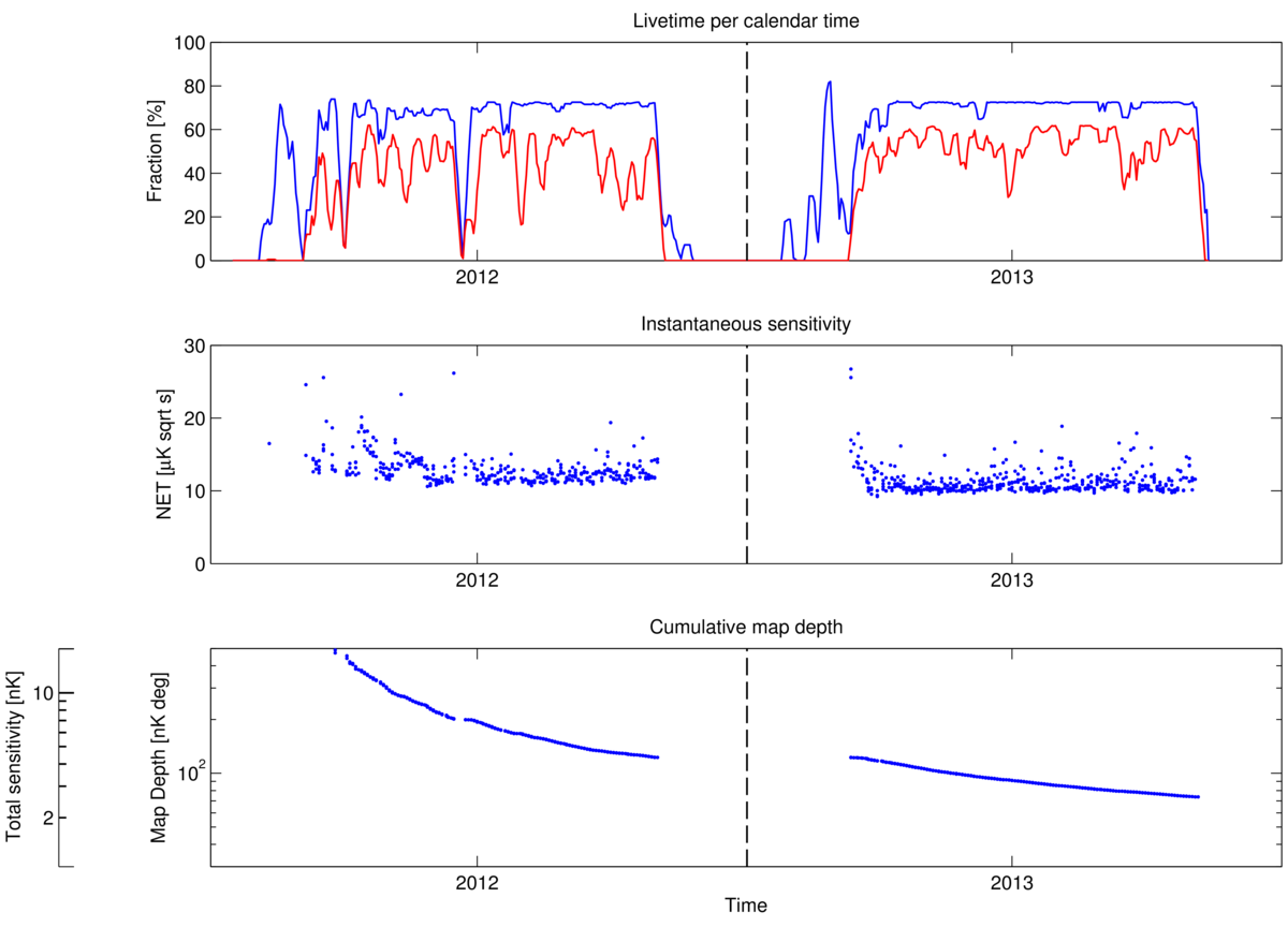
Figure 2: The Keck Array 2012–2013 150 GHz data set. The top panel
shows the fraction of calendar time the telescopes were observing. The
red line represents the fraction of time preserved after all data selection
cuts are implemented. The middle panel shows the instantaneous sensitivity
of the full Keck Array. The bottom panel shows the cumulative map depth
as calculated over each phase (10 hr of data).
|
PDF / PNG |
| Keck Array T, Q, U maps |
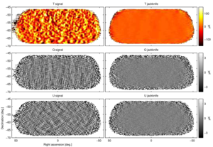 |
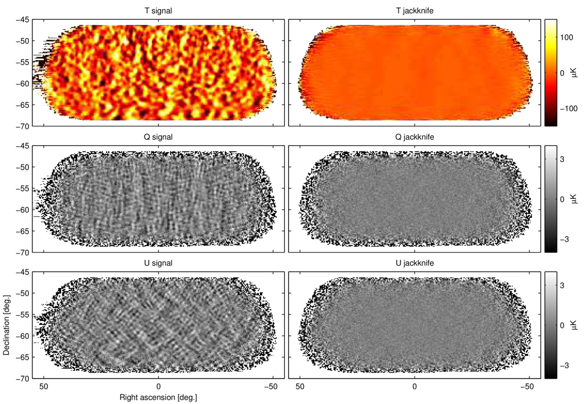
Figure 3: Keck Array T, Q, U maps.
The left column shows the basic signal maps with 0.25° pixelization
as output by the reduction pipeline.
The right column shows difference (jackknife) maps made with the
first halves of the 2012 and 2013 seasons and the second halves.
No additional filtering other than that imposed by the instrument beam
(FWHM 0.5°) has been done.
Note that the structure seen in the Q and U signal maps is as expected
for an E-mode dominated sky.
|
PDF / PNG |
| Power spectrum jackknife |
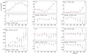 |
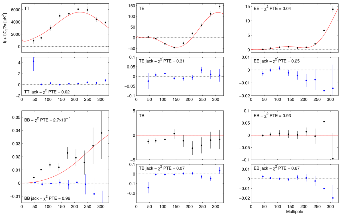
Figure 4: Keck Array power spectrum results for signal (black points)
and early/late season jackknife (blue points).
The solid red curves show the lensed-ΛCDM theory expectations.
The error bars are the standard deviations of the
lensed-ΛCDM+noise simulations and hence contain no sample variance
on any additional signal component.
The probability to exceed (PTE) the observed value of a simple
χ2 statistic for the 9 band powers is given (as evaluated against the simulations).
Note that the band powers of the auto spectra of the simulations are approximately
χ2 distributed, with the lowest ℓ-bin only containing ∼9 effective degrees of freedom.
This increases the probability of an outlier point in comparison to a Gaussian distribution.
The observed distribution for the cross spectra are more symmetric than the χ2 distributions but have similarly increased tails.
This is fully reflected in the quoted PTE value.
Also note the very different y-axis scales for the jackknife spectra
(other than BB).
See the text for additional discussion of the BB spectrum.
(Note that the calibration procedure uses EB to set the overall polarization angle
so TB and EB as plotted above cannot be used to measure astrophysical
polarization rotation.)
|
PDF / PNG |
| E-mode and B-mode maps |
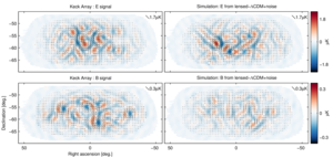 |
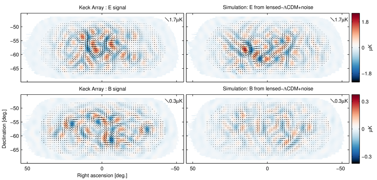
Figure 5: Left: Keck Array apodized E-mode and B-mode maps filtered to 50<ℓ<120.
Right: The equivalent maps for the first of the lensed-ΛCDM+noise simulations.
The color scale displays the E-mode scalar and B-mode pseudoscalar patterns
while the lines display the equivalent magnitude and orientation of linear polarization.
Note that the E-mode and B-mode maps use different
color/length scales.
|
PDF / PNG |
| Jackknife PTE distributions |
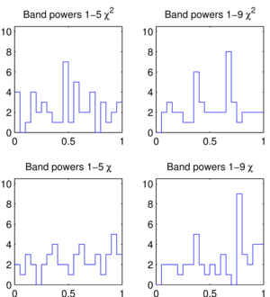 |
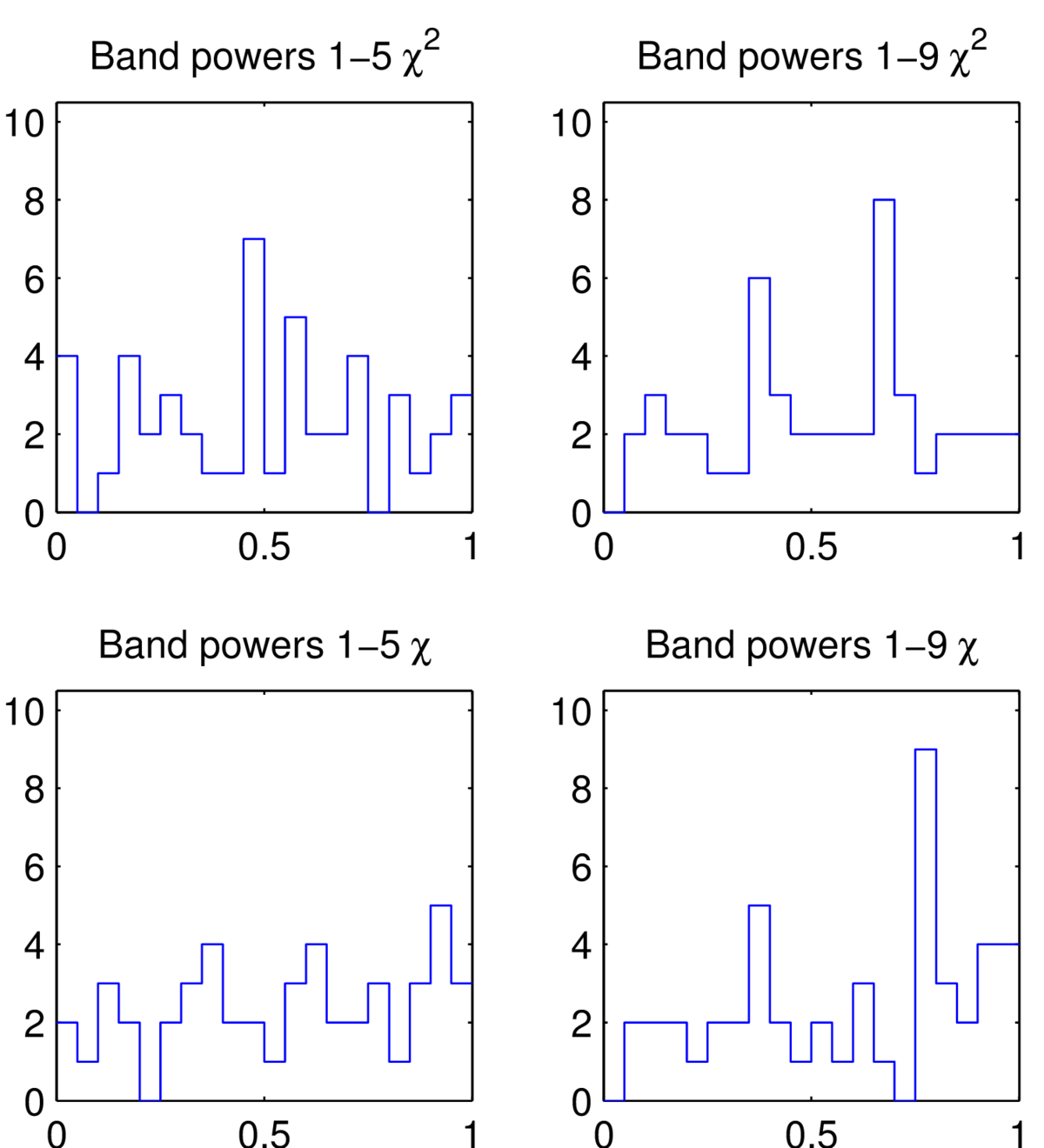
Figure 6: Distributions of the jackknife χ2 and χ PTE values over the tests and spectra given in Table 4.
|
PDF / PNG |
| BB spectra from T-only input simulations |
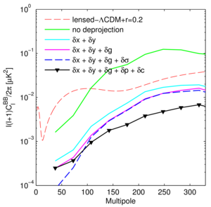 |
Figure 7: BB spectra from T-only input simulations using
the measured per channel beam shapes
compared to the lensed-ΛCDM+r=0.2 spectrum.
From top to bottom the curves are (i) no deprojection,
(ii) deprojection of differential pointing only (δ x + δ y),
(iii) deprojection of differential pointing and differential gain of the
detector pairs (δ x + δ y + δ g),
(iv) adding deprojection of differential beam width (δ x + δ y +
δ g + δσ), and
(v) differential pointing, differential gain, and differential
ellipticity (δ x + δ y + δ g + δ p + δ c).
This last curve represents an upper limit only to the residual contamination.
|
PDF / PNG |
| Comparison of BICEP2 and Keck Array BB spectra |
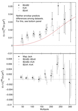 |
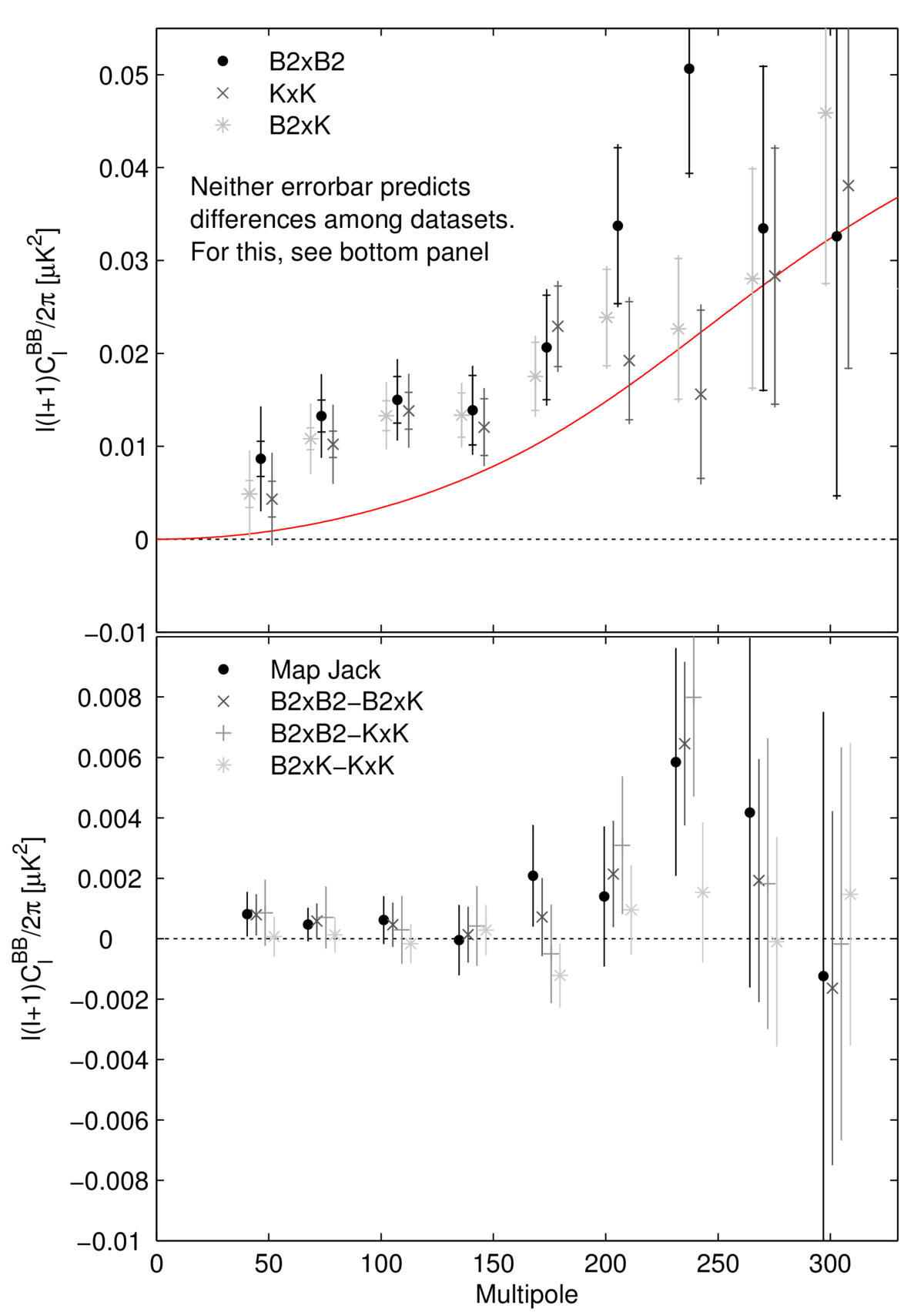
Figure 8: Upper: The Keck Array BB auto spectrum,
the BICEP2 auto spectrum, and the cross spectrum taken between the two.
The inner error bars are the standard deviation of the lensed-ΛCDM+noise simulations,
while the outer error bars also contain excess power at low-ℓ.
(For clarity the Keck Array and cross spectrum points
are offset horizontally.)
Lower:
Four compatibility tests between the B modes measured by
BICEP2 and Keck Array.
The “map jack” takes the difference of the Q and U maps,
divides by a factor of two,
and calculates the BB spectrum.
The other three sets of points are the differences of the spectra shown in
the upper panel divided by a factor of four.
In each case the error bars are the standard deviation of the
pairwise differences of signal+noise simulations
which share common input skies. Comparison of any one of
these sets of points with null is an appropriate test
of the compatibility of the experiments—see text for details.
All tests show good consistency between BICEP2 and Keck Array,
particularly in the lowest five band powers.
|
PDF / PNG |
| BB power spectrum of combined BICEP2 and
Keck Array maps |
 |
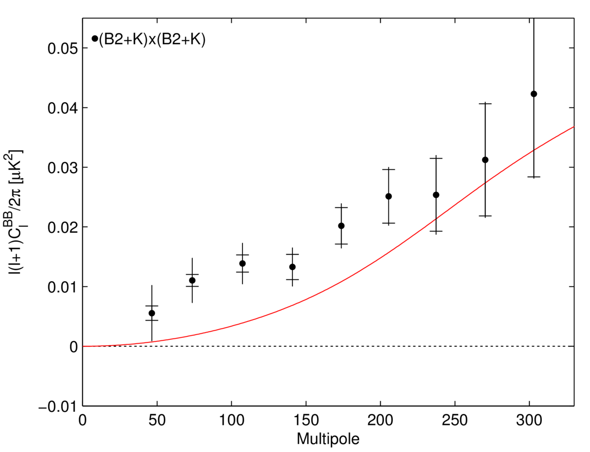
Figure 9: The BB power spectrum of combined BICEP2 and
Keck Array maps.
The inner error bars are the standard deviation of the lensed-ΛCDM+noise simulations,
while the outer error bars also contain excess power at low-ℓ.
|
PDF / PNG |