-
BK-III: Instrumental Systematics
The BICEP2 Collaboration, ApJ 814, 110, 2015
| Figures | Download Bundle | ||
|---|---|---|---|
| Map coverage of a single detector pair |  |
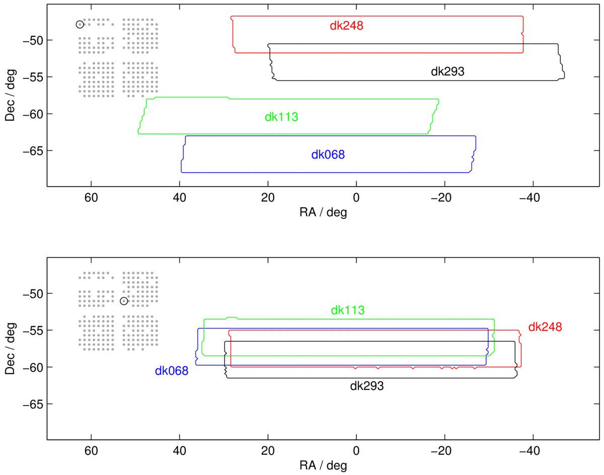
Figure 1: Map coverage of a single BICEP2 detector pair located (top panel) near the edge of the focal plane and (bottom panel) near the center of the focal plane. The coverage at different deck angles overlaps significantly for central detectors but not at all for edge detectors. The inset (not drawn to scale) indicates the location of the detector pair in the focal plane. | PDF / PNG |
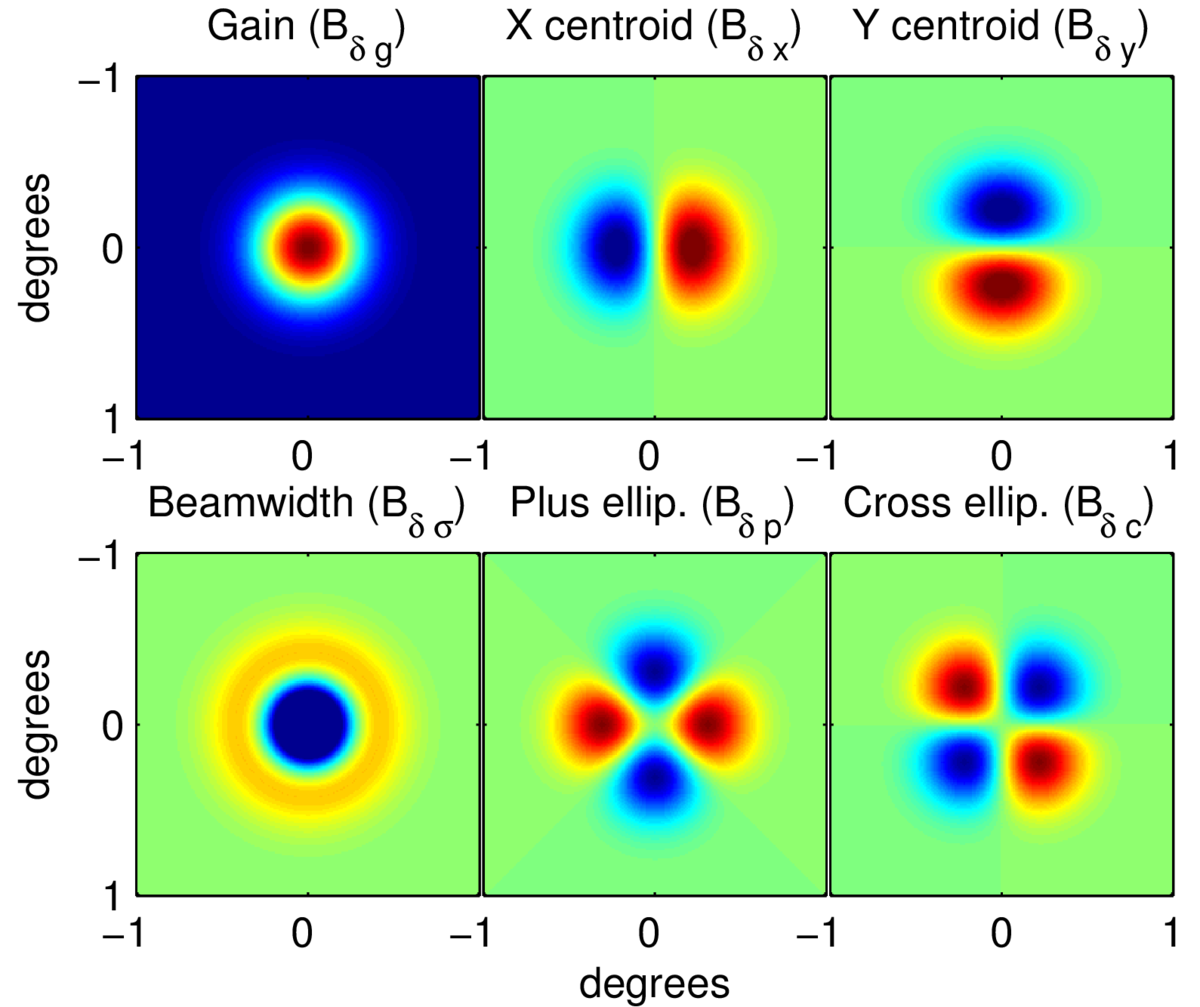
| Differences of elliptical Gaussian beams |  |
Figure 2: Differences of elliptical Gaussian beams. The total difference beam is the linear combination of these modes. Differential gain and beamwidth produce monopole symmetric difference beams, differential pointing a dipole symmetric difference beam, and differential ellipticity a quadrupole symmetric difference beam. These difference beams couple to different derivatives of the underlying CMB temperature field. | PDF / PNG |
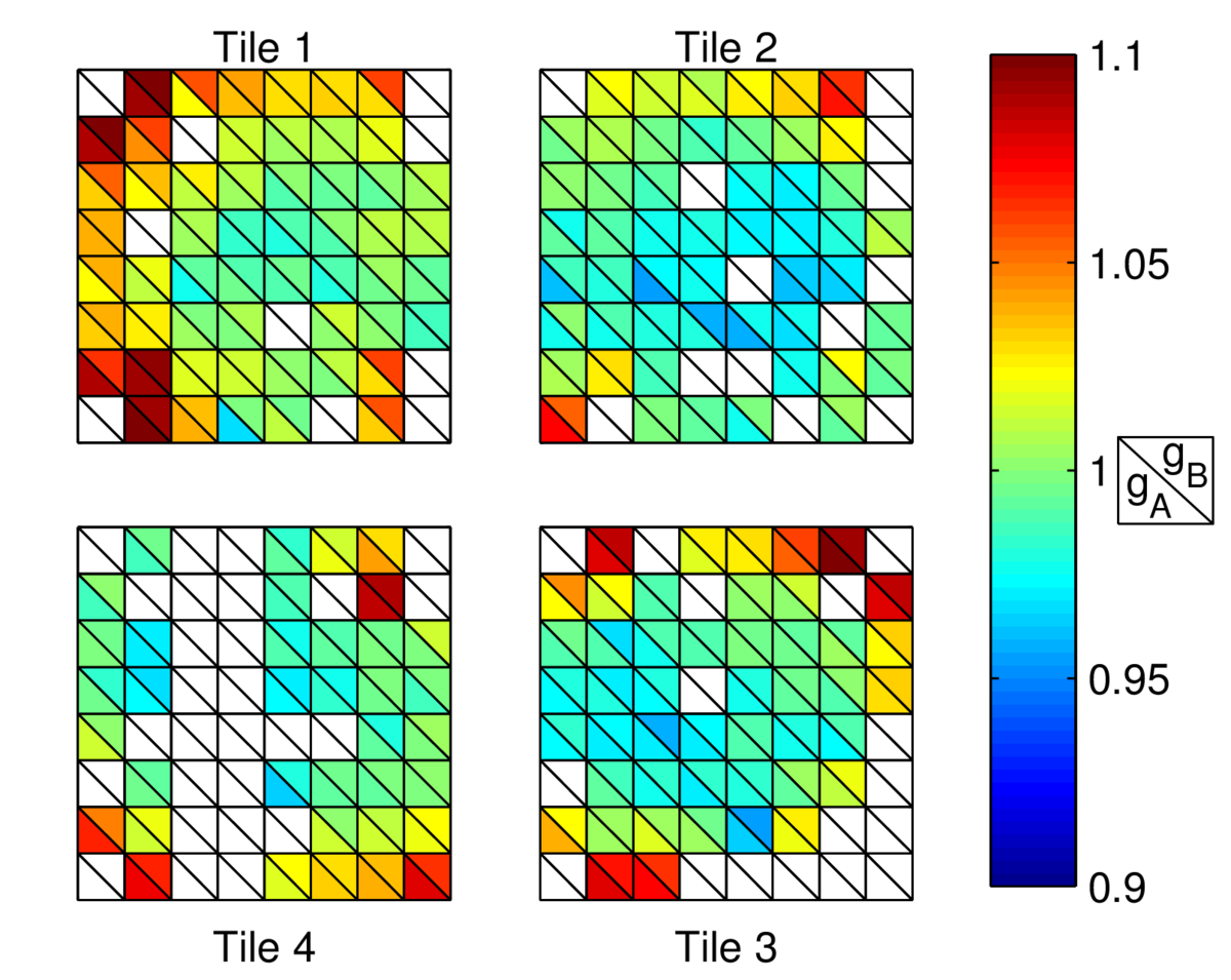
| Measured absolute gain for each detector | 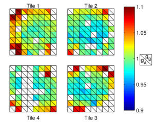 |
Figure 3: Measured absolute gain for each detector included in BICEP2's maps. The gains are normalized such that the median gain is one. The distribution within the focal plane is represented schematically. Each detector pair is depicted as a small square. The A (B) member of a detector pair is depicted as the lower (upper) triangle of the square. | PDF / PNG |
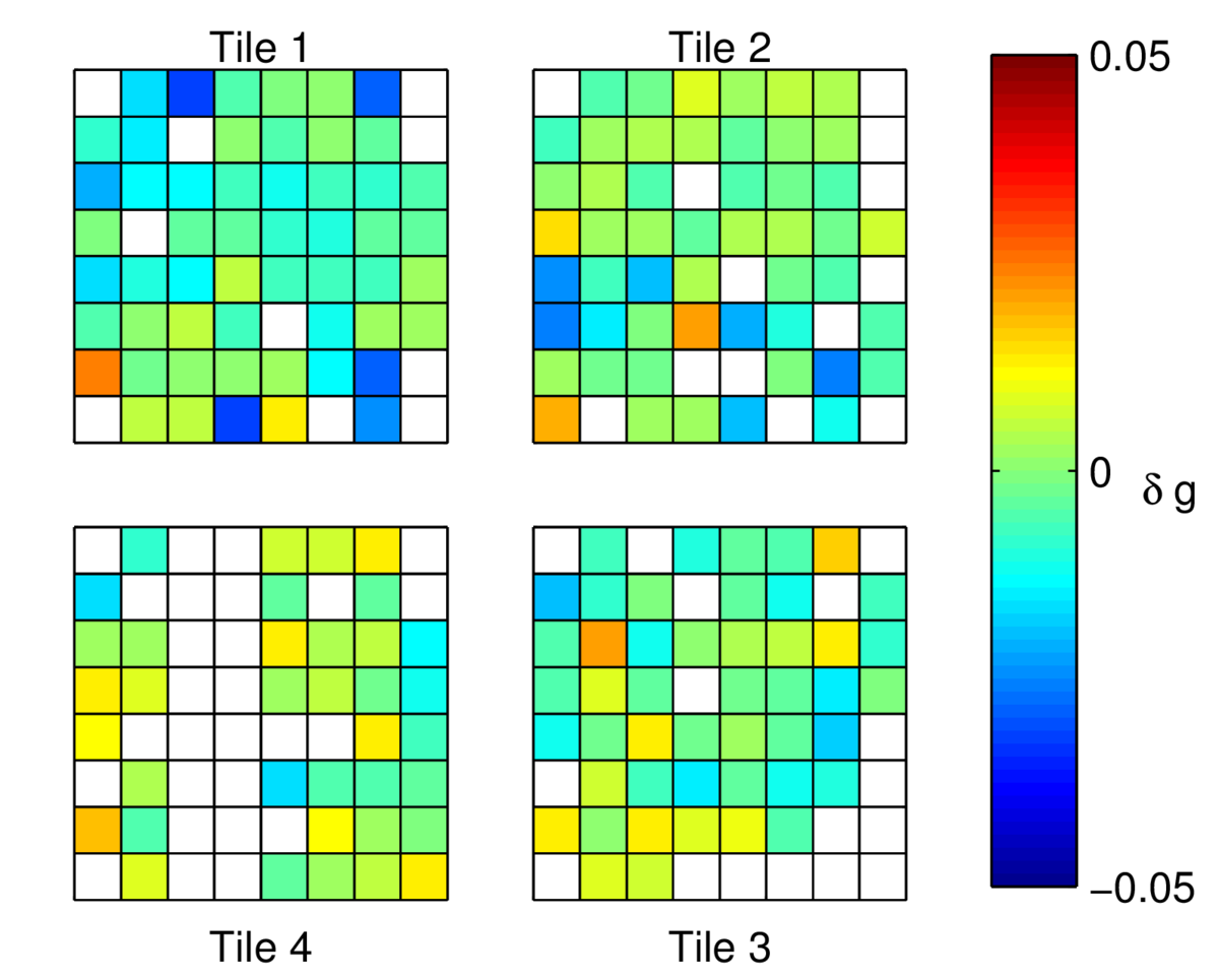
| Measured differential gain | 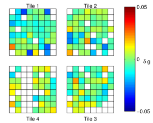 |
Figure 4: Measured differential gain for each detector pair included in BICEP2's maps. | PDF / PNG |
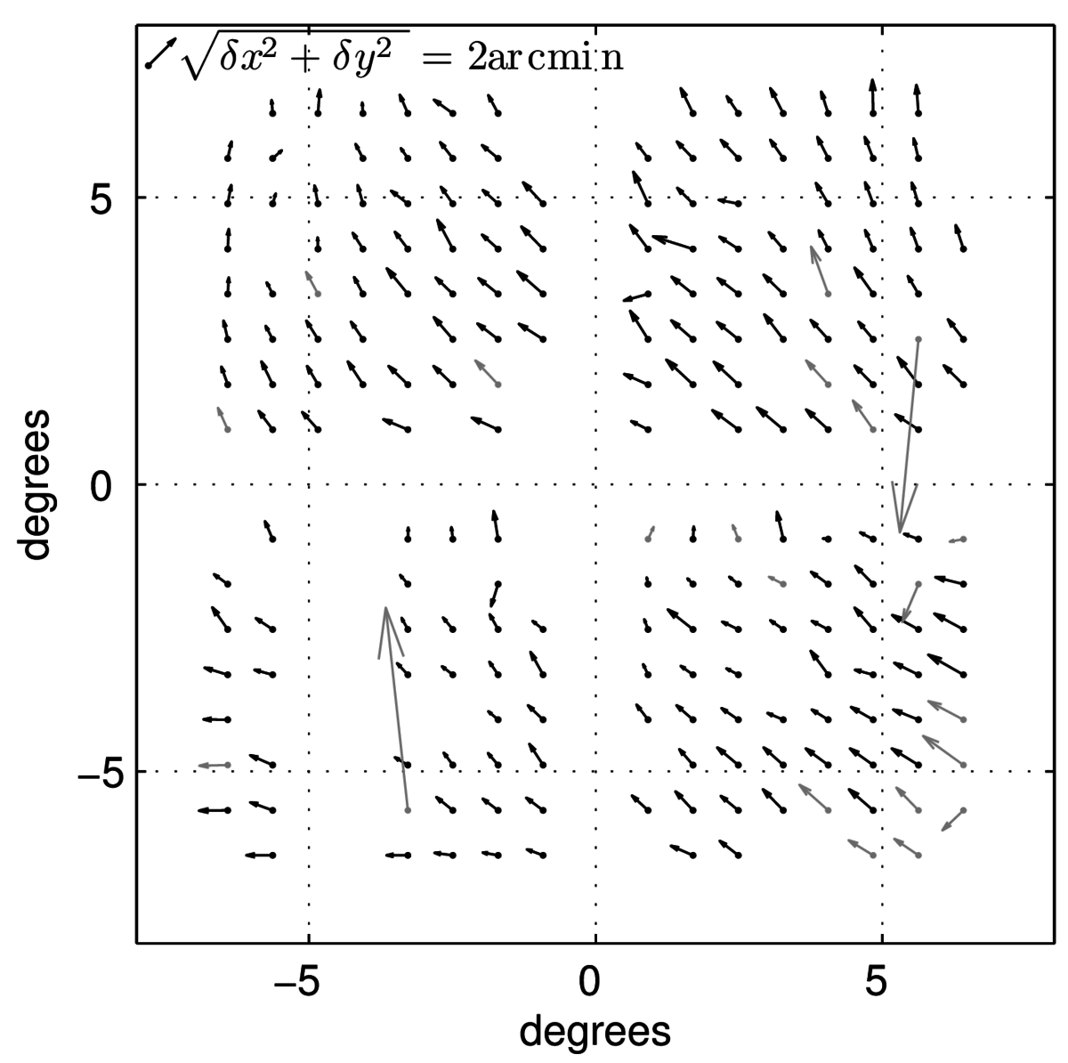
| Differential pointing in the BICEP2 focal plane | 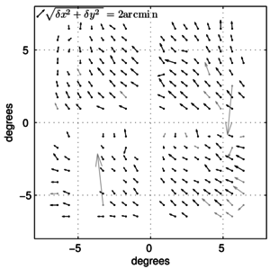 |
Figure 5: Differential pointing in the BICEP2 focal plane as projected onto the sky. As drawn, the vectors originate at the nominal beam center and point from detector B to detector A. Their magnitudes are drawn ×20 for display purposes. All functioning pairs are plotted, but grayed out vectors indicate detector pairs that are excluded from the final maps. | PDF / PNG |
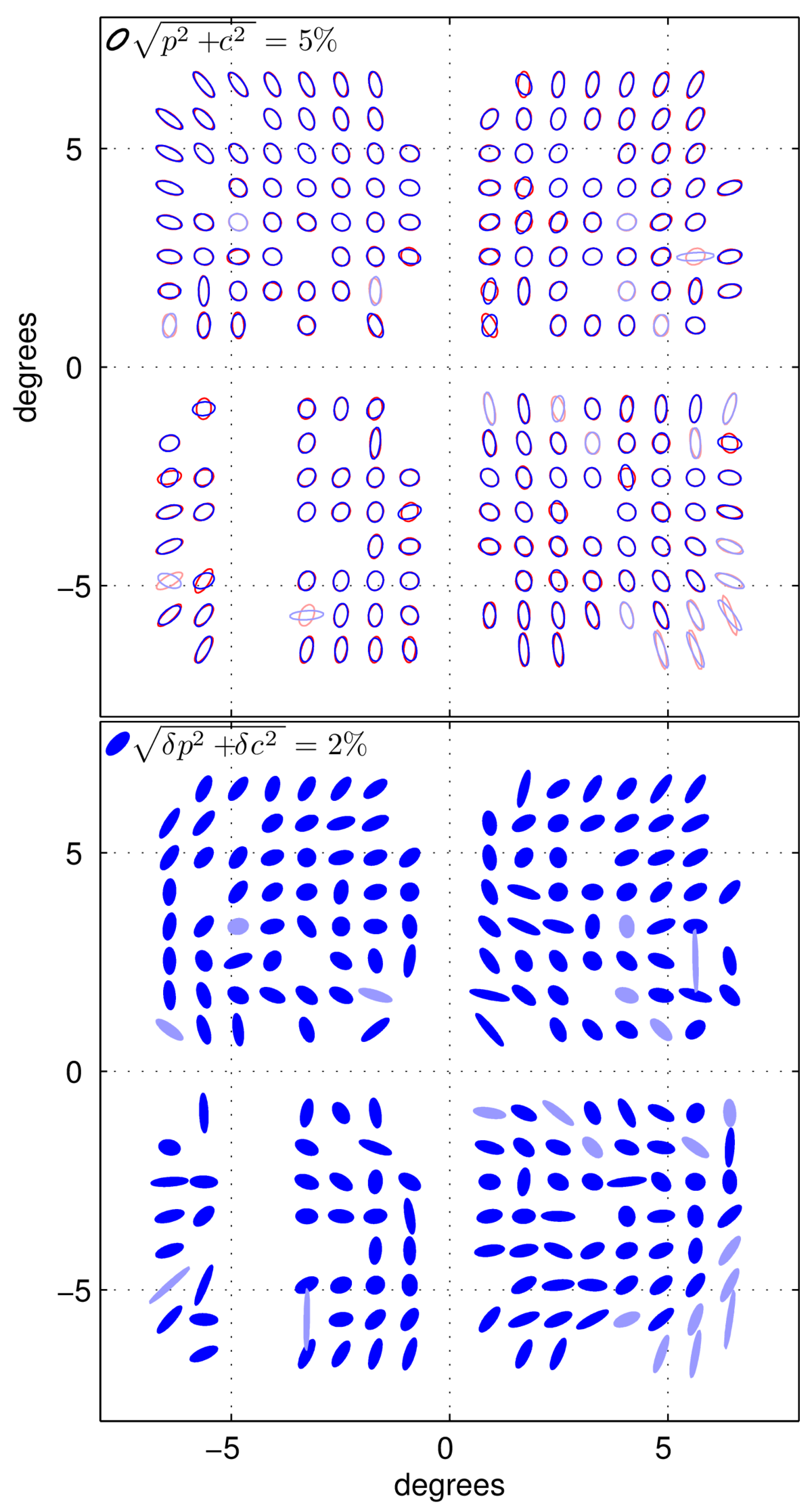
| Beam ellipticity | 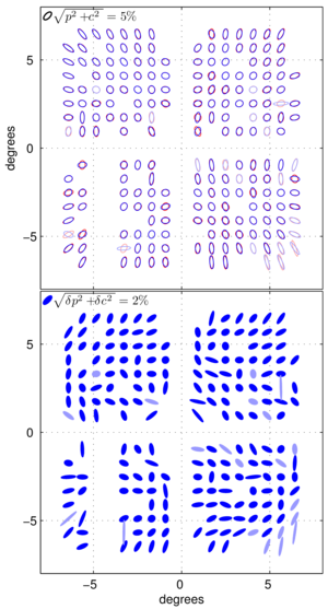 |
Figure 6: Top: per-detector beam ellipticity in the BICEP2 focal plane as projected onto the sky. Ellipticity is exaggerated for clarity. Red and blue denote A and B members of a detector pair, respectively. All functioning pairs are plotted, but light colors indicate detectors that are excluded from the final map. Bottom: per-pair differential ellipticity. The orientation of the ellipse indicates the orientation of the difference beam quadrupole. Detector polarization angles are aligned with the horizontal and vertical axes. | PDF / PNG |
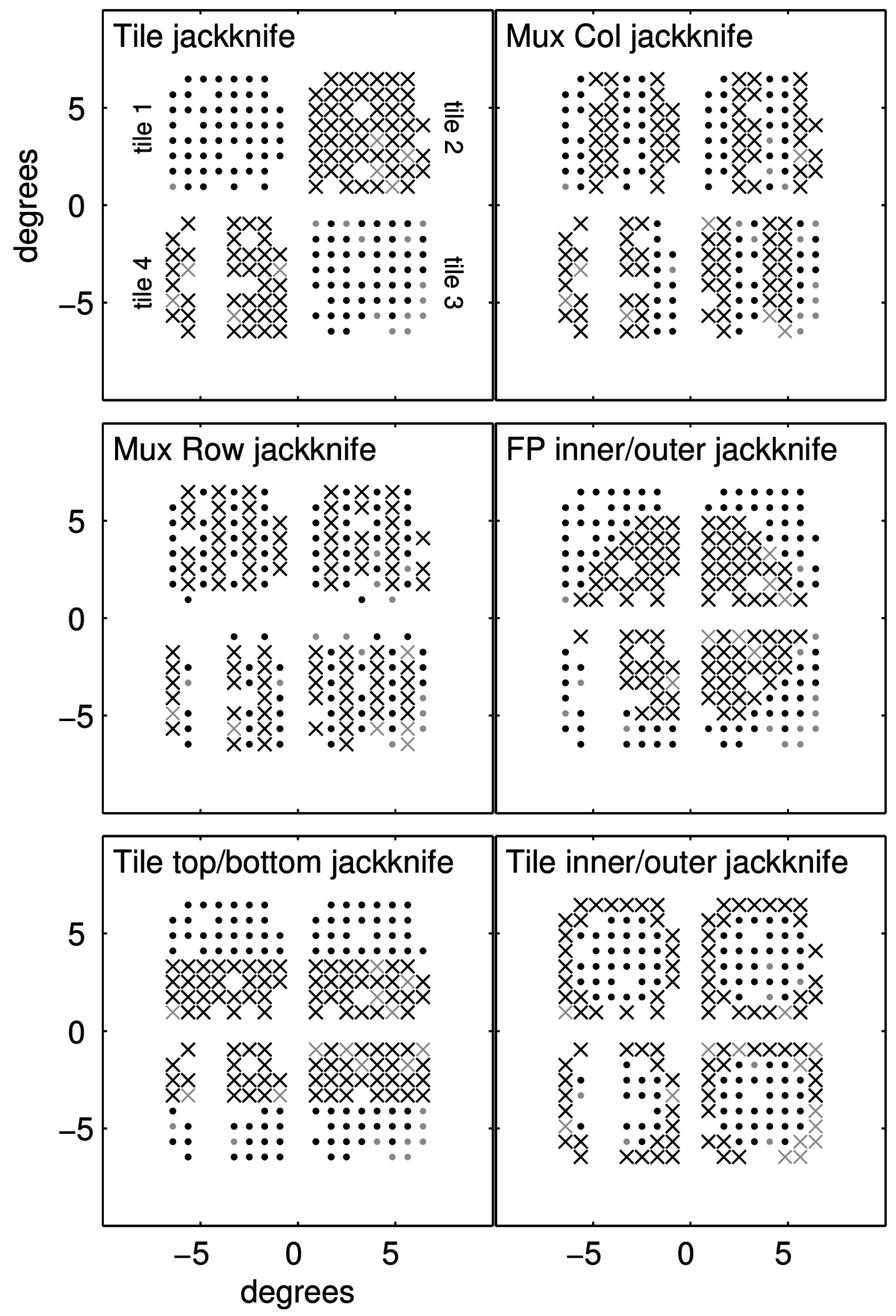
| Map of detector pair selection jackknife splits | 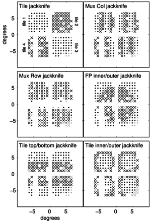 |
Figure 7: Map of the BICEP2 focal plane projected onto the sky illustrating detector pair selection jackknife splits. Dots denote detector pairs that are coadded to form one half of the jackknife split; X's denote detector pairs coadded to form the other half. All functioning pairs are shown. Light gray symbols indicate pairs that are excluded from the final map. | PDF / PNG |
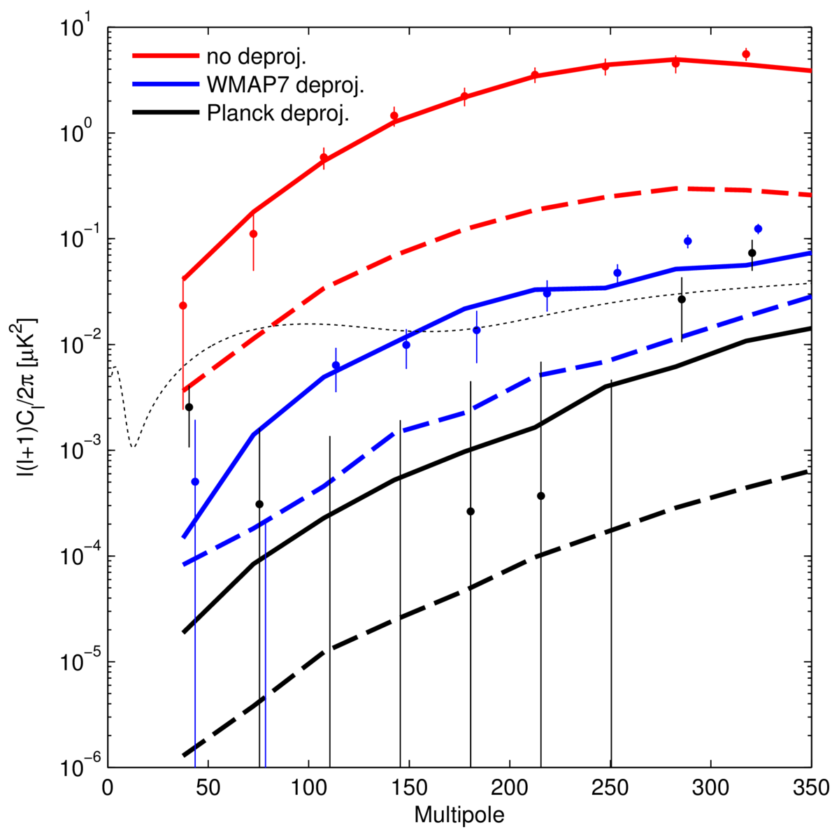
| BICEP2's deck jackknife bandpowers |  |
Figure 8: Points with error bars are BICEP2's deck jackknife bandpowers with (red) no deprojection, (blue) differential pointing deprojected with a WMAP7 V-band template, and (black) differential pointing deprojected with a Planck 143 GHz template, with error bars taken as the standard deviation of ΛCDM plus instrumental noise simulations that include BICEP2's measured differential pointing. The solid lines are the corresponding simulated deck jackknife spectra, computed as the mean of 50 noiseless simulations of ΛCDM T and BICEP2's measured differential pointing, deprojected with templates containing simulated template noise. The dashed lines show the simulated non-jackknife, signal BB leakage. The dotted line shows a lensed ΛCDM + r=0.2 spectrum for reference. | PDF / PNG |
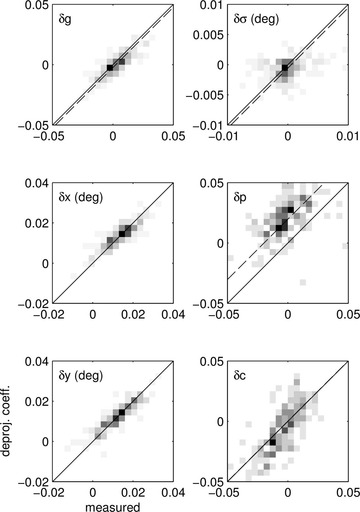
| Differential beam parameters |  |
Figure 9: Differential beam parameters measured from far-field beam maps (horizontal axis) and from template regression as used in deprojection (vertical axis), shown as 2-d histograms over detector pairs. (Differential gains are determined from cross-correlation of individual detector T maps with Planck.) The solid line has slope one and y-intercept zero. The dashed line has slope one but has been offset vertically by the bias in the recovered deprojection coefficients predicted from simulation. The scatter and bias in the observed relation is broadly consistent with that predicted from signal-plus-noise simulations. | PDF / PNG |
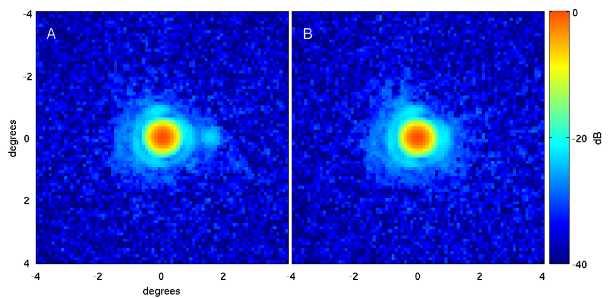
| Composite beam map | 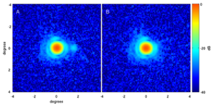 |
Figure 10: Composite beam map for a representative detector pair, showing the A and B beams. The coordinate system is centered on the mean pair-centroid. The expected crosstalk feature with ~-25 dB amplitude is visible in the A detector on the horizontal axis at a distance of ~+1.7° from the beam center. The first Airy ring is visible at a radius of ~1°. The difference beam (not shown) is dominated by a dipole structure. | PDF / PNG |
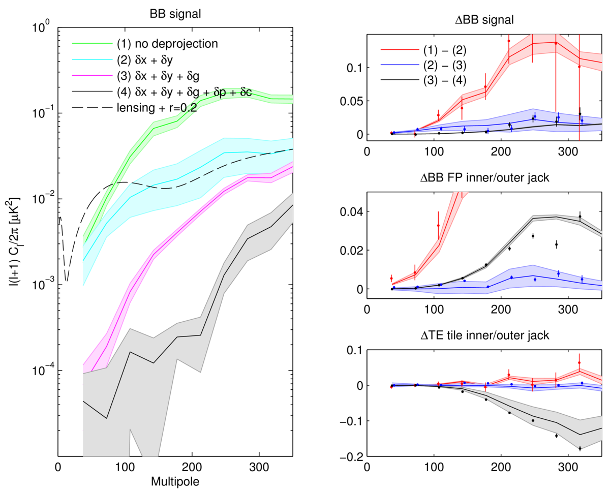
| BB contamination predicted from beam map simulations and changes in bandpowers with different deprojection choices | 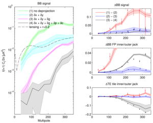 |
Figure 11: Left panel: BB contamination predicted from beam map simulations of BICEP2's measured main beams (temperature only simulations using the Planck HFI 143 GHz T map convolved with measured, per-detector beam maps). The shaded bands indicate the 1σ uncertainty of the contamination given the sensitivity of the beam maps and gain mismatch measurements. The colors correspond to different choices of deprojection: (1) no deprojection; (2) deprojection of differential pointing (δ x + δ y); (3) deprojection of differential pointing and differential gain (δ x + δ y + δ g); and (4) deprojection of differential pointing, differential gain, and differential ellipticity (δ x + δ y + δ g + δ p + δ c). Right panels: Changes in bandpowers with different deprojection choices for: (top) the BB signal spectrum, (middle) the BB focal plane inner/outer jackknife, and (bottom) the TE tile inner/outer jackknife. The solid lines and shaded bands again indicate the mean and 1σ uncertainty of the predicted leakage given the sensitivity of the beam maps and gain mismatch measurements. The points with error bars are the real data bandpower differences, with error bars computed as the rms of BICEP2's standard, lensed-ΛCDM signal plus instrumental noise simulation set. | PDF / PNG |
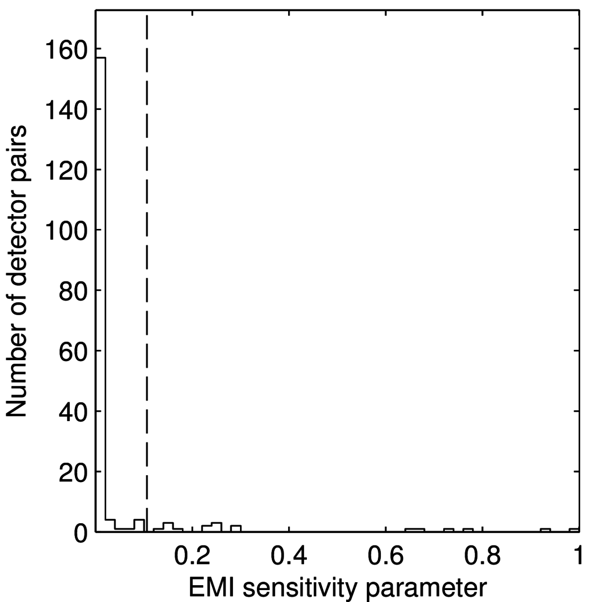
| EMI sensitivity parameter |  |
Figure 12: EMI sensitivity parameter for all detector pairs included in BICEP2's maps. The parameter is proportional to the contribution of possible EMI from a given detector pair to BICEP2's polarization power spectra. The dashed line indicates the cut threshold used in constructing the EMI sensitivity pair exclusion test. | PDF / PNG |
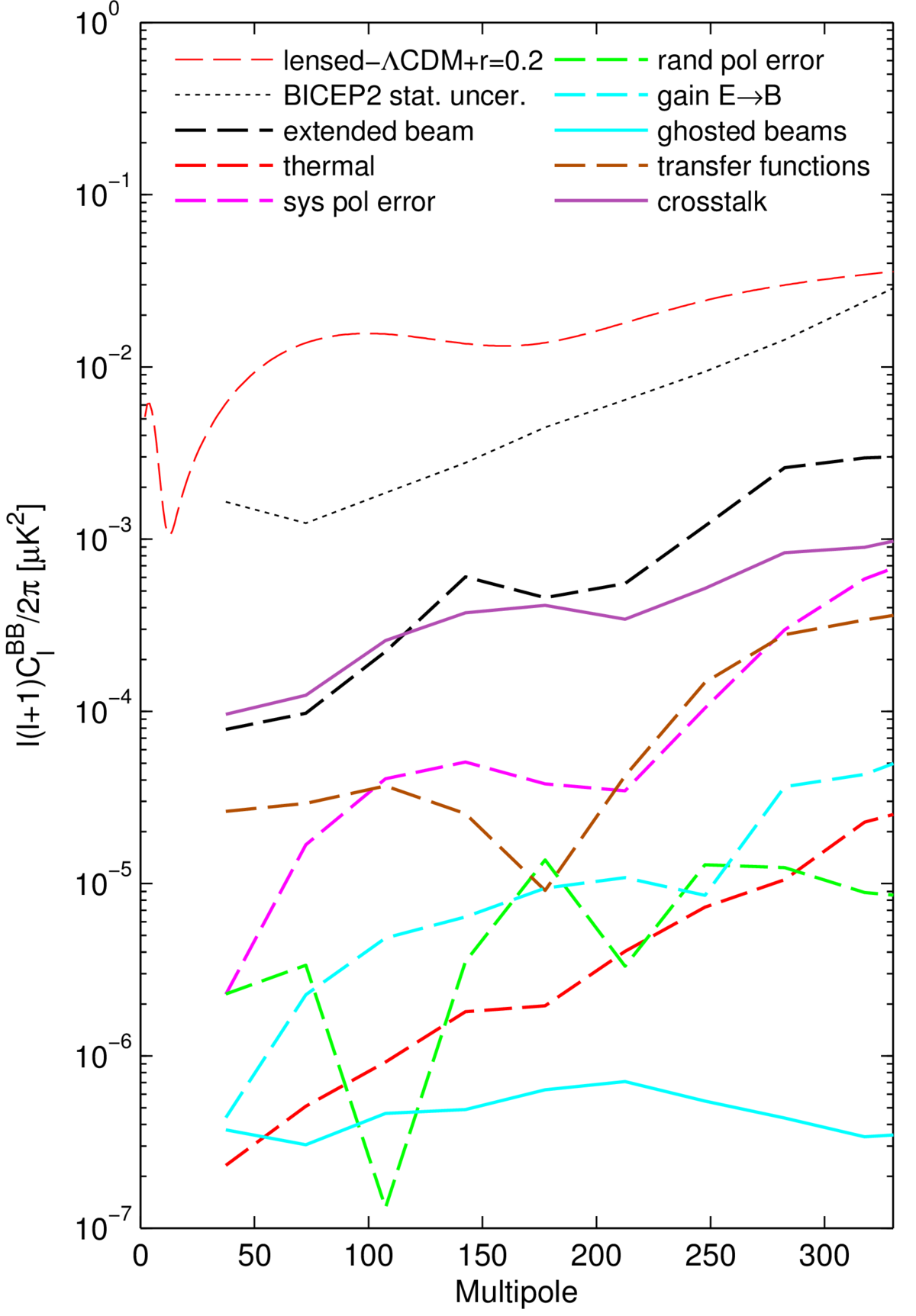
| Estimated levels of systematics |  |
Figure 13: Estimated levels of systematics as compared to a lensed-ΛCDM+r=0.2 spectrum. Solid lines indicate expected contamination. Dashed lines indicate upper limits. All systematics are comparable to or smaller than the extended beam mismatch upper limit, which is smaller than BICEP2's statistical uncertainty. | PDF / PNG |
| Illustration of T→P leakage resulting from differential pointing | (a)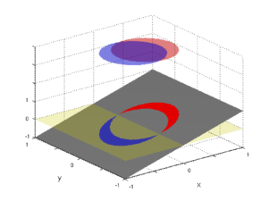 (b)
(b) |
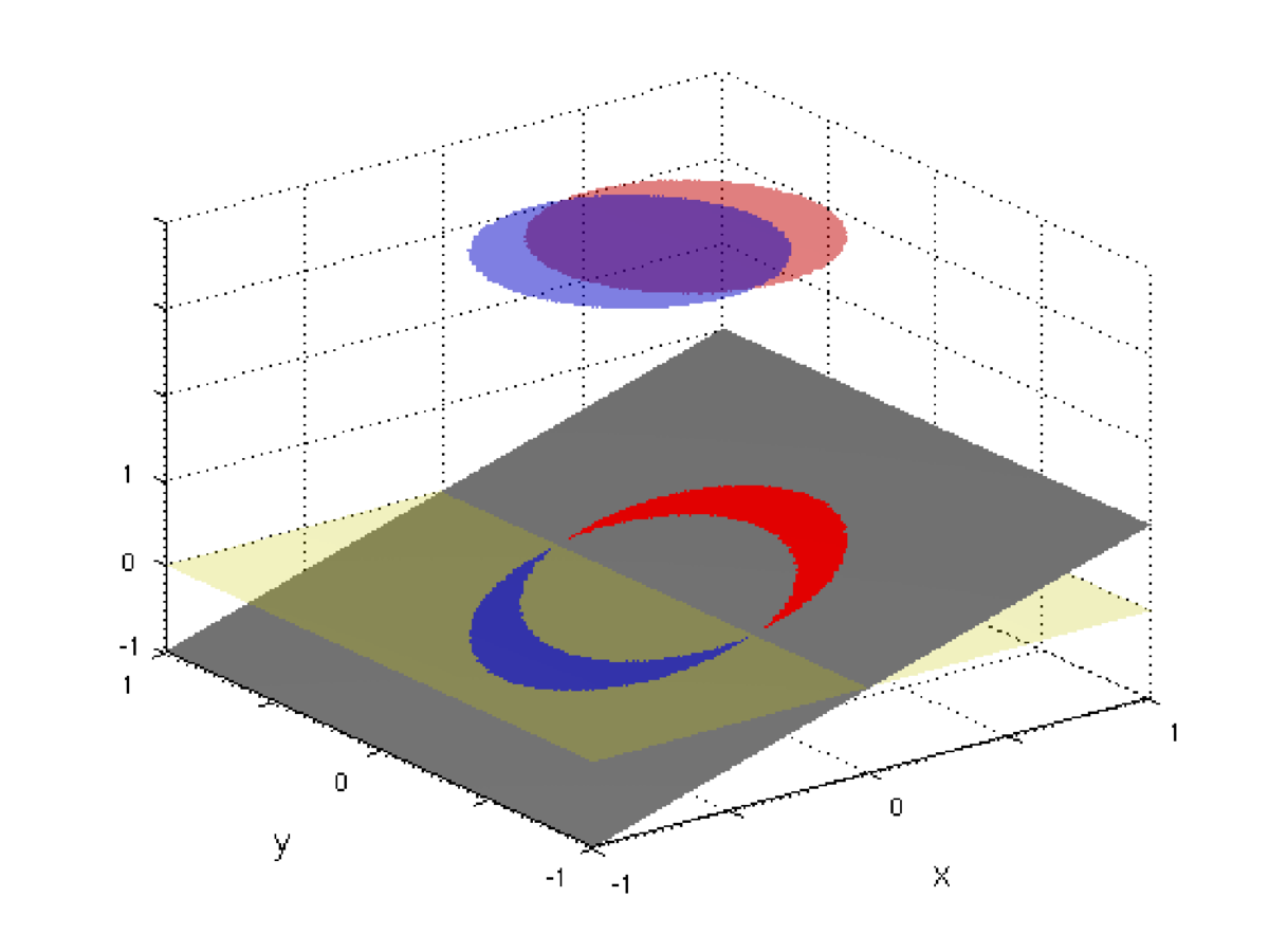
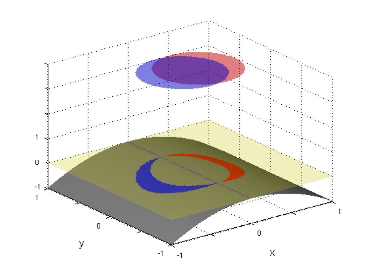
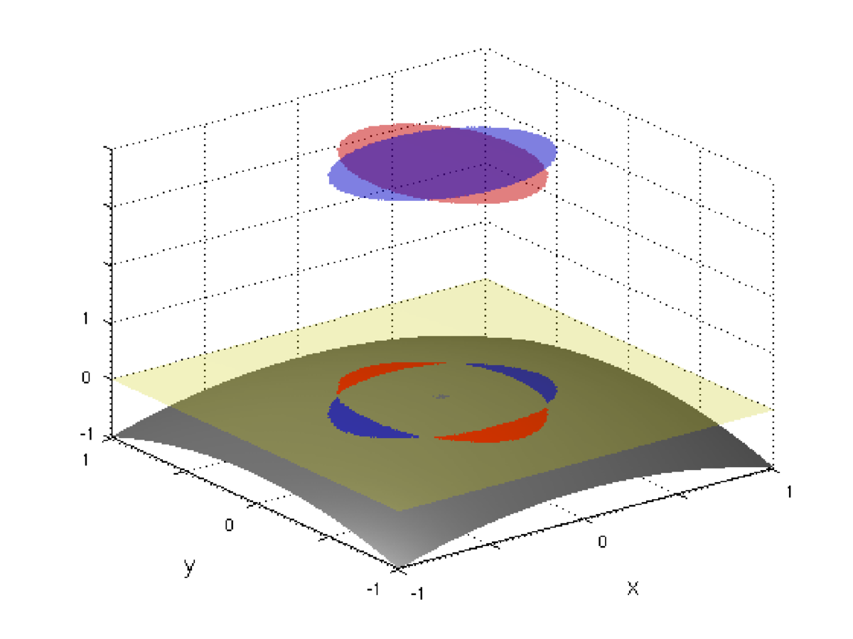
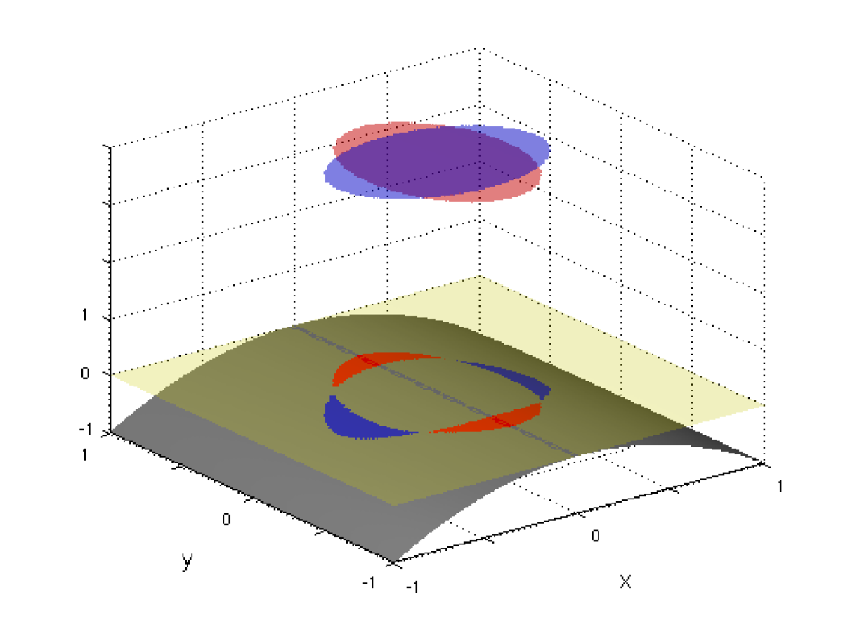
Figure 14: Illustration of T→P leakage resulting from differential pointing. The gray plane represents a T sky with (a) ∇xT>0, ∇2xT=0, and (b) ∇xT=0, ∇2xT<0. The red and blue circles represent contour slices through the circular Gaussian beams of the A and B members of a detector pair, respectively. The non-overlapping area is projected onto the T plane. The transparent green plane at z=0 is simply for reference. The scenario in (a) leaks T→P while (b) does not. |
(a)PDF / PNG (b)PDF / PNG |
| Illustration of T→P resulting from differential beamwidth |
(a) (b)
(b)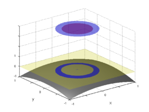 |
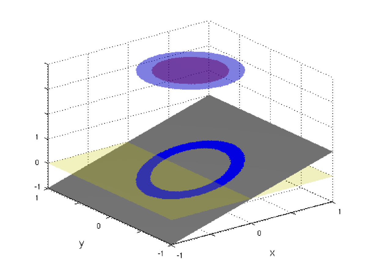
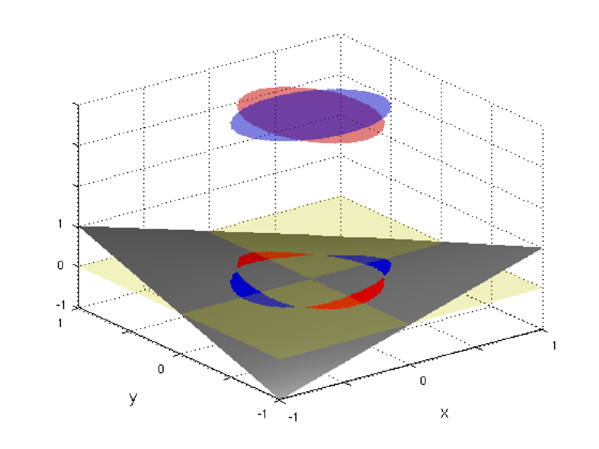
Figure 15: Illustration of T→P resulting from differential beamwidth. The gray plane represents a T sky with (a) ∇xT>0, ∇2xT=∇2yT=0, and (b) ∇xT=0, ∇2xT=∇2yT<0. The scenario in (b) leaks T→P while (a) does not. |
(a)PDF / PNG (b)PDF / PNG |
| Illustration of T→P leakage resulting from differential plus-ellipticity |
(a)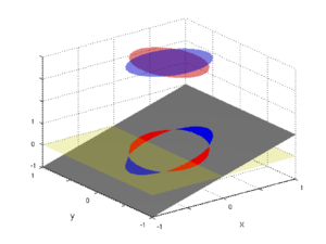 (b)  (c)  (d) 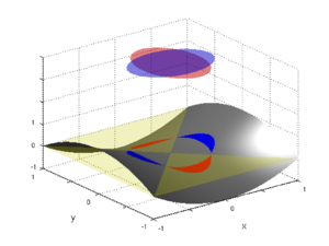 (e) 
|
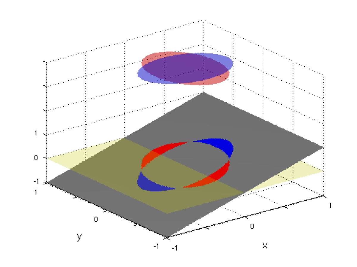
Figure 16: Illustration of T→P leakage resulting from differential plus-ellipticity. The gray plane represents a T sky with (a) ∇xT>0, ∇2xT=∇2yT=∇x∇yT=0; (b) ∇xT=∇x∇yT=0, ∇2xT=∇2yT<0; (c) ∇xT=∇x∇yT=∇2yT=0, ∇2xT<0; (d) ∇xT=∇x∇yT=0, ∇2yT<0<∇2xT; (e) ∇xT=∇2xT=∇2yT=0, ∇x∇y≠0. Only the scenarios in (c) and (d), which have a non-zero difference of orthogonal second derivatives, leak T→P. |
(a)PDF / PNG (b)PDF / PNG (c)PDF / PNG (d)PDF / PNG (e)PDF / PNG |
History
- 2015-02-02: Posted BK-III: Instrumental Systematics figures.